MATLAB SOFTWARE
ABOUT MATLAB
The name MATLAB stands for “matrix laboratory”. MATLAB is a high-performance technical computing. It integrates computation, visualization, and programming in an easy-to-use environment where problems and solutions are expressed in familiar mathematical notation. Typical uses include:
Math and computation
Algorithm development
Modeling, simulation, and prototyping
Data analysis, exploration, and visualization
Scientific and engineering graphics
Application development, including graphical user interface building
MATLAB is an interactive system whose basic data element is an array that does not require dimensioning. This allows you to solve many technical computing problems, especially those with matrix and vector formulations, in a fraction of the time it would take to write a program in a scalar non-interactive language such as C or Fortran.
MATLAB features a family of application-specific solutions called toolboxes. Very important to most users of MATLAB, toolboxes allow you to learn and apply specialized technology. Toolboxes are comprehensive collections of MATLAB functions (M-files) that extend the MATLAB environment to solve particular classes of problems. Areas in which toolboxes are available include signal processing, control systems, neural networks, fuzzy logic, wavelets, simulation, and many others.
THE MATLAB SYSTEM:
The MATLAB system consists of five main parts:
Development Environment: This is the set of tools and facilities that help you use MATLAB functions and files. Many of these tools are graphical user interfaces. It includes the MATLAB desktop and Command Window, a command history, and browsers for viewing help, the workspace, files, and the search path.
The MATLAB Mathematical Function Library: This is a vast collection of computational algorithms ranging from elementary functions like sum, sine, cosine, and complex arithmetic, to more sophisticated functions like matrix inverse, matrix eigenvalues, Bessel functions, and fast Fourier transforms.
The MATLAB Language: This is a high-level matrix/array language with control flow statements, functions, data structures, input/output, and object-oriented programming features. It allows both "programming in the small" to rapidly create quickly and dirty throwaway programs, and "programming in the large" to create complete large and complex application programs.
Handle Graphics: This is the MATLAB graphics system. It includes high-level commands for two-dimensional and three-dimensional data visualization, image processing, animation, and presentation graphics. It also includes low-level commands that allow you to fully customize the appearance of graphics as well as to build complete graphical user interfaces on your MATLAB applications.
The MATLAB Application Program Interface (API): This is a library that allows you to write C and Fortran programs that interact with MATLAB. It includes facilities for calling routines from MATLAB (dynamic linking), calling MATLAB as a computational engine, and for reading and writing MAT-files.
MATLAB WORKSPACE:
The MATLAB workspace consists of the set of variables (named arrays) built up during a MATLAB session and stored in memory. You add variables to the workspace by using functions, running M-files, and loading saved workspaces. For example, if you type
t = 0:pi/4:2*pi;
y = sin(t);
The workspace includes two variables, y and t, each having nine values.
ABOUT SIMULINK:
Simulink is a software package for modeling, simulating, and analyzing dynamical systems. It supports linear and nonlinear systems, modeled in continuous time, sampled time, or a hybrid of the two. Systems can also be multirate, i.e., have different parts that are sampled or updated at different rates.
For modeling, Simulink provides a Graphical User Interface (GUI) for building models as block diagrams, using click-and-drag mouse operations. With this interface, you can draw the models just as you would with pencil and paper. This is a far cry from previous simulation packages that require you to formulate differential equations and difference equations in a language or program. Simulink includes a comprehensive block library of sinks, urges, linear and nonlinear components, and connectors. You can also customize and create your own blocks.
Models are hierarchical, so you can build models using both top-down and bottom-up approaches. You can view the system at a high level, then double-click on blocks to go down through the levels to see increasing levels of model detail. This approach provides insight into how a model is organized and how its parts interact. After you define a model, you can simulate it, using a choice of integration methods, either from the Simulink menus or by entering commands in MATLAB's command window. The menus are particularly convenient for interactive work, while the command-line approach is very useful for running a batch of simulations (for example, if you are doing Monte Carlo simulations or want to sweep a parameter across a range of values). Using scopes and other display blocks, you can see the simulation results while the simulation is running. In addition, you can change parameters and immediately see what happens. The simulation results can be put in the MATLAB workspace for post processing and visualization.
Model analysis tools include linearization and trimming tools, which can be accessed from the MATLAB command line, plus the many tools in MATLAB and its application toolboxes. And because MATLAB and Simulink are integrated, you can simulate, analyze, and revise your models in either environment at any point
DESIGN AND STUDY OF FILTERS
DESIGN STEPS FOLLOWED
MATLAB offers varieties of toolboxes using that we can easily design the required digital filter and can observe its phase and magnitude characteristics; construct realization structure of the designed filter; analyze working of the filter.
To design a filter and analyze it we followed below mentioned steps:
Using “Filter Designer And Analyzer” window we designed our required filter. To open this window type “fdatool” in Command Window and press “Enter”. The obtained filter coefficients (i.e. numerator and denominator coefficients) are noted.
Using “Filter Realization Wizard” window we have constructed the filter structure by inputting filter coefficients and selecting the appropriate form. To open this window type “dspfwiz” on Command Window and press ‘enter’ key. Using ‘Launch Pad’ also we can open this window. Select DSP Blockset from the ‘Launch Pad’ and click on the +ve mark corresponding to it. A drop down list opens up. From this list select ‘Filter Realization Wizard’ and double click on it. This opens that window. The constructed structure appears as a subsystem model. A double click on the subsystem block opens the filter structure in Simulink window, which can be simulated.
Using Simulink block library function generator, oscilloscope and MUX are connected to the filter structure. Using Simulink debugger the structure is simulated and the results are observed on the oscilloscope.
IIR FILTER DESIGN ISSUES
We restrict our discussion to the design and analysis of IIR filters only, even though FIR filters provide linear phase throughout the frequency range. In application of our project phase angle variation is of no importance; if phase angle variation is also important then automatically discussion orients towards FIR filters.
Before directly going into the analysis of IIR filters let us have a glance over Shannon’s sampling theorem.
“A signal containing maximum frequency f1Hz may be completely represented by regularly spaced samples, provided the sampling rate ‘fs’ is at least 2f1 sample per second.”
i.e. fs=2f1 Nyquist sampling rate
If signal is sampled at less than 2f1 rate, aliasing error occurs. Signal is then represented with distortion, which depends on the degree of aliasing. To avoid such distortions use antialiasing filter, a low pass filter with cutoff frequency at f1(or fs/2).
Because of above reason designing any digital filter at higher frequency side becomes difficult owing to higher sampling rate and its generation. Hence we need to restrict ourselves to lower frequency side. Further discussion on these issues will be elaborated in respective filter design studies to forth come.
IIR Low pass And High pass Filter Design Issues
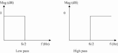
The ideal response of low pass and high pass filters is as shown in Figure 1
Practically such sharp roll off is not achievable. Using MATLAB we can easily design these filters and simulate it. Even at higher frequencies (like 40KHz) “simulink” work satisfactorily. The filter nicely exhibits passband and stopband action.
In most of the applications lowpass/highpass filters are used at lower frequencies with increased order, so that sharp roll-off is achieved.

Figure 1
IIR Bandpass Filter Design And Its Implementation
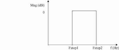
Ideally bandpass filter should have a perfect passband as shown in the Figure 2
But practically such a sharp cutoff at passband edges is not possible. Therefore practically we aim towards a response, which has as much sharper role-off as possible, so that “channel selection” is performed noiselessly. Chebyshev and elliptic filters provide very good response in this regard. Hence we select Chebyshev type of filter for our study and analysis as it provides satisfactory bandpass characteristics

Figure 2
Chebyshev Type-II Filter Design
Filter parameters are as shown bellow-
Order = 2
Sampling frequency Fs = 100KHz
Fstop1 = 39KHz
Fstop2 = 41KHz
Astop= 60db
Input the above parameters to the respective places of “Filter Design & Analysis Tool”. After completing this click on ‘Design Filter’ button. This creates the required filter .To observe the response (step or frequency or impulse) click on the respective icon of the toolbar. Toolbar also has icons to observe pole-zero plot, group delay, filter coefficients etc. Thus the obtained filter coefficients are as follows:
Numerator (b) Denominator (a)
0.000062910740701 1.000000000000000
0.000000000000000 1.621131129004091
-0.000062910740701 0.999874178518599
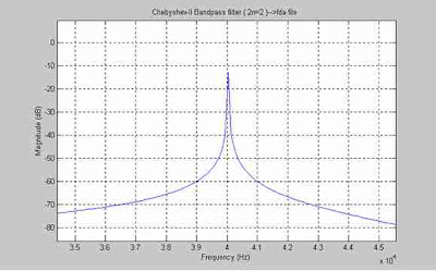
For the above parameters magnitude response can be observed by clicking on corresponding icon of the toolbar. The corresponding frequency response is as shown bellow in Figure 3.

For the same above filter parameters MATLAB program is written in a M-file to create chebyshev type-II bandpass filter.
The program is as follows….
File name:cheby.m
clc;
clear all;
close all;
As=60; %stopband attenuation
wp1=3.8e+004; %lower cutoff frequency
wp2=4.2e+004; %higher cutoff frequency
n=1; %order
fs=100000; %sampling frequency
wn=[wp1 wp2]/(fs/2); %Nyquist frequency
[b,a] = cheby2(n,As,wn); %compute filter coefficients
[h,f]=freqz(b,a,fs/2); %compute frequency response
mag=20*log10(abs(h)); %get magnitude response
subplot (2,1,1);
plot(f*(fs/2)/pi, mag);grid; %plot response with grid lines
ang=angle(h); %get phase response
subplot(2,1,2);
plot(f*(fs/2)/pi,ang);grid; %plot response with grid lines
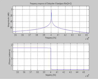
Run this program either by pressing F5 key on keyboard or select ‘Run’ from debug menu. The obtained magnitude and phase response is as shown bellow in Figure 4

Figure 4
For both of the above filter designs, the corresponding filter realization structure of Direct Form –2 is as shown in Figure 5. This can be created using “Filter Realization Wizard” by inputting filter coefficients.
From the frequency response curves (Figure 4) of the above filter we can analyze the filter.
Thus the Chebyshev type-2 filter designed with n=1(implies order 2n=2) and pass band =2KHz(implies +/- 1KHz from 40KHz) has very sharp (like a pulse) passband and also not exactly centered at 40KHz.Owing to this shift of passband either towards the left or right side of frequency domain, the center frequency may get attenuated or noise signals may creep through the filter resulting in a distorted output. Another possibility is suppose by some means frequency of input signal itself varies from its central value then filter may pass unwanted signals and it may attenuate the original signal itself creating a noisy output. This may due to the inconsistency of function generator. We can’t say even crystal oscillator can produce exactly 40KHz signal. It may vary a little (+/-100Hz) due to variation of temperature, pressure, applied voltage etc.
Therefore we need a filter, which has a passband, so that even though center frequency varies from its value, the signal is reproduced faithfully at the output and all other unwanted signal frequencies are completely attenuated.
We can meet the requirements by changing the filter parameters like order, pass band, edge frequency or stop band attenuation. But it is found that keeping order n=1 even though we increase pass band range and decrease stop band attenuation, don’t yield satisfactory result instead it just attenuated pass band itself.
Therefore to improve the filter performance the only left option is to increase the filter order and this is what done in most of the practical cases. We adjust the pass band frequency so that around 500 to 800 Hz pass band with minimum attenuation is obtained.
Using “Filter Design & Analysis Tool” we can do this and by noting down the filter coefficients we can realize filter structure.
CHEBYSHEV TYPE-II FILTER DESIGN WITH INCREASED ORDER
Filter parameter: n = 4 (2n = 4=> n =2)
Fs = 100000Hz.
Fstop1 = 38000Hz.
Fstop2 = 41800Hz.
Astop = 40dB.
Let the file name given to this filter be ‘filter40.fda’
The obtained magnitude response is as shown in Figure 6 and the corresponding filter coefficients are as follows,
Numerator (b) Denominator (a)
b(0)=0.010045097978992. a(0)=1.000000000000000.
b(1)=0.031677960303578. a(1)=3.205603560877597.
b(2)=0.044659670697279. a(2)=4.521600439016961.
b(3)=0.031677960303578. a(3)=3.129988499837994.
b(4)=0.010045097978992. a(4)=0.953386226509250.
EFFECT OF TRUNCATION OF COEFFICIENT ON FILTER RESPONSE
Digital signal processing algorithms are realized either with special purpose digital hardware or as programs for a general-purpose digital computer. In both cases the numbers and coefficients are stored in finite-length registers. Therefore, coefficients and numbers must be quantised by truncations or rounding before they can be stored.
The following errors arise due to quantisation of numbers,
Input quantisation error.
Product quantisation error.
Coefficient quantisation error.
The conversion of a continuous time input signal into digital value produces an error, which is known as input quantisation error arises due to the representation of the input signal by a fixed number of digits in the A/D conversion process.
Product quatisation errors arise at the output of a multiplier. Multiplication of ‘a’ and ‘b’ bit with ‘ab’ bit coefficient results a product having ‘2b’ bits. Since ‘ab’ bit register is used, the multiplier output must be rounded or truncated to ‘b’ bits, which produces an error.
The filter coefficients are computed to infinite precision in theory. If they are quantised, the frequency response of the resulting filter may differ from the desired response and sometimes the filter may fail to meet the desired specifications. If the poles of the desired filter are close to the unit circle, then those of the filter with quantized coefficients may lie just outside the unit circle, leading to the unstability.
The other errors arising from quantization are round off noise and limit cycle oscillations.
It can be understood from the above points that quantisation error due to A/D conversion process is difficult to minimize below certain limits in any sophisticated processor. Using higher sampling rate we can minimize this error.
Using processors with higher word length registers can minimize product quantisation errors. As length of the operating registers become more and more error becomes less and less. If floating point arithmetic is supported in processor then this error can be eliminated to a very large extent.
Now let us analyze the filter40.fda named filter for different truncated values.
In this file, the coefficients obtained are 64-bit length (i.e. 16 decimal number excluding decimal point). Notice that these are the coefficients, which are obtained by designing the filter in ‘ Filter design & Analysis tool’.
To find out what is the effect of truncating the coefficient data, we use M-file program ‘cheby.m’. Here we directly feed the filter coefficients to the ‘freqz’ command as shown below:
Clc;
Clear all;
Close all;
b=[ b(0) b(1) b(2) b(3) b(4) ]; %fill numerator coefficients
a=[ a(0) a(1) a(2) a(3) a(4) ]; %fill denominator coefficients
[h, f]=freqz (b,a,fs/2);
If you don’t put semicolon at the end of the line where numerator and denominator coefficients are written and you run the program, you can find that at the command window, these coefficients are rounded up to 4th decimal point. The software itself automatically does the truncation of data. The resultant frequency response by this truncated data is same as that of obtained with non-truncated data with hardly noticeable differences.
The rounding up of numerator and denominator to third decimal point causes below response:
Numerator (b) denominator (a)
0.010 1.000
0.032 3.206
0.045 4.522
0.032 3.130
0.010 0.953
The rounding up of numerator and denominator to second decimal point causes heavy variation in pass band attenuation as shown in Figure 8.
Numerator (b) Denominator (a)
1.00
3.21
4.52
3.13
0.95
Rounding up of filter coefficient to the first decimal point abruptly changes frequency characteristics of the filter.
From the above discussion it follows that truncating the filter coefficients to 4th decimal point yields good acceptable frequency characteristics and hence can be implemented in hardware.
The filter structure for the above filter is as shown below in Figure 9.
SIMULATING THE FILTER STRUCTURE
To simulate the above filter structure, it has to be modified a little bit.
First open “Simulink Library Browser”. Select and drag the ‘Sine Wave’ block from the source library to the window where the structure is created. Similarly ‘Scope’ is dragged from the ‘Sinks’ library and the ‘Mux’ is dragged from the ‘Signals & Systems’ library. Substitute ‘input’ by ‘sine Wave’ block, output by ‘Mux’ and ‘Scope’ block. By double clicking on each block we can get the properties of each block. For example: double click on “sine wave” block. This will open a window wherein we can write frequency of the signal, signal voltage, sampling time etc. In the same way “mux” and scope can be configured.
After connecting all these blocks click on “start” icon on the toolbar to start simulation. Options are there to “pause” the simulation, “stop” the simulation etc. We can also see the simulation status on “simulink debugger” window. Double click on the “scope” block. This opens the oscilloscope where we can observe the input and output waveforms.
The study and analysis of simulation of the above filter structure as well as many other filter structures (like Cheby type-1, 2 Butterworth –lowpass/highpass) are carried out successfully.
One thing that is particularly noticeable is that for higher frequencies simulation of filter structure takes more time compared to simulation of filter structure at lower frequencies. Effect of truncation of coeffients can also be observed on the ‘Scope’ and also works as the study has been done in earlier sections.
References
“Digital Signal Processing” By Sanjit K.Mitra
“Digital Signal Processing” By P.Ramesh Babu
“Digital Filters” By T.J.Terrel And E.T.Powner
“BASIC Digital Signal Processing” By Gordon B. Lockart And Barry M.G.Cheetham
“Digital Signal Processing” By Alan V.Oppenheim And Ronald W.Schafer
“DSP Microprocessors: Advances and Automotive Applications” By Subra Ganeshan And Dr.Gopal Arvamudhan
www.mathworks.com


Tula's International School is known to be one of the residential school and best boarding school in India The school is affiliated with Central Board of Secondary Education (CBSE) and has been awarded with numerous accolades in the field of education.
ReplyDeleteTula's International School Boarding School in India